Features Soil Summit 2019 Fertility and Nutrients
SWAT maps: the foundation of variable-rate fertility

When talking about variable rates, start with the end in sight. You have to have a picture in your mind of what the zone maps are going to look like before you even make them. I’m going to build that picture for you today. Put the right rate in the right zone.

Point one, you must get the zone maps right. I’m going to spend probably 90 per cent of my time on that one right there. If you don’t get your zone maps right, you’re done. I’ll spend maybe just 10 per cent of the time on getting the fertilizer rates right. Normally, I would spend a lot more, but I think, in the interest of time, I’m just going to spend times on zone maps today.

What causes variability? Everything, right? There are tons of things that cause variability. Fertility is just one little part of all the variability that’s going on out on the field.

The best way to get a map of all of the variability together, typically, is some type of an image of your field, whether that’s satellite image, yield maps or other ways. The point is these are tools that, a given point in time, if you take a shot of your crop in June, it’ll show you everything that affected your crop in June. Cutworms ate the hills. The hills didn’t come up that good because it was dry. You mudded in the depressions. Too much residue in some spots. That’s what it’s going to show. Everything.

So, this is just a drone image that Greg flew for us for a particular field at Wadena I’m going to spend a lot of time on today. Wadena is about three hours east of Saskatoon here in the Quill Lakes Watershed. We’ve got eight years of correlated imagery here. We built a yield potential map, and I’m just going to show this to you in 3D because it’s much easier to understand.

Photos courtesy of Cory Willness/CropPro Consulting.

If you look at this picture, you can see the high yielding areas are all typically mid-slopes in this field and are the most consistent land in that area. It’s not the first thing to flood. It’s not the first thing to dry out. It doesn’t have salinity. It’s guaranteed crop country in that area. The tops of the hills are medium yield potential. You look at some of these depressions and they are medium yield potential. Some areas are saline spots with medium yield potential. So, it’s putting a whole bunch of factors together that, yes, they’re medium yield potential, but they’re not all the same thing, right? These maps are a good representation of historical yield.

Now, having said that, 50 per cent of the time when we make those yield potential maps, whether it’s long-term historic yields or long-term historic images, there’s no correlation between the years. In other words, there’s so much variability from the high and low areas of yield from year to year that you can’t even relate one year to the other. This is an accurate yield potential map, but, now, is that a zone map? It’s just not the starting point. It isn’t the foundation for zones.

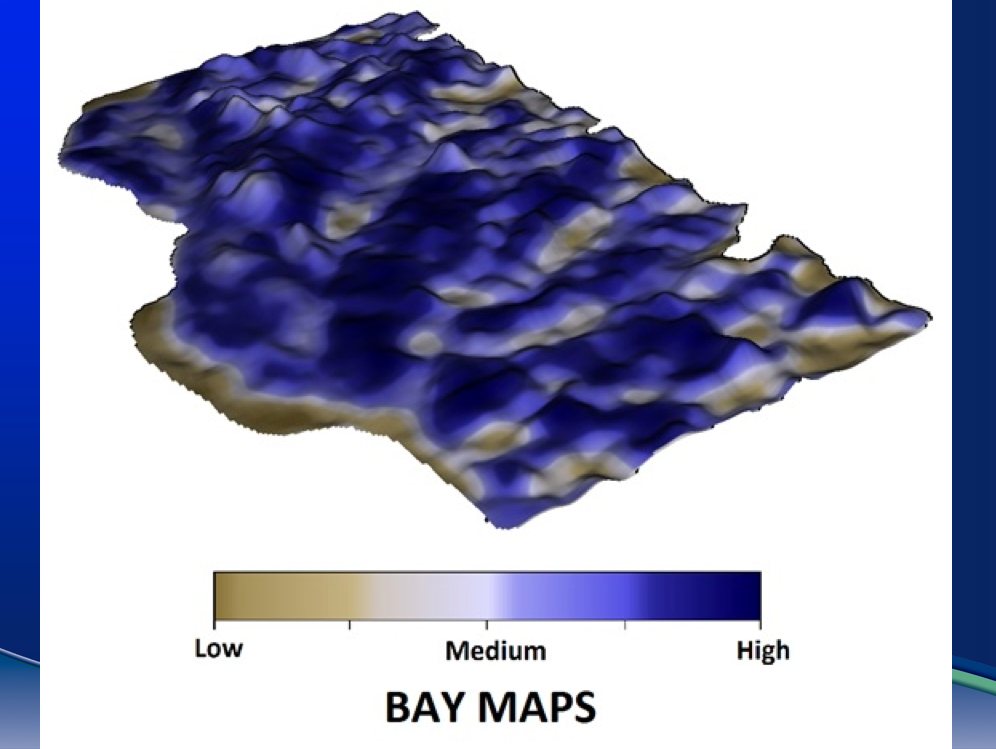
So, how do we get focused in on zones then? We’ve got all of this variability. In my opinion, these are the three primary things that you need to get a picture of in the field, to understand what your fertilizer response variability is going to be. Those are soil, water and topography. Notice that they’re all interrelated, right? Topsoil depth and organic matter levels, are related to topography. Different soil properties, like texture, influence how much water can be stored, and are also at different spots in the landscape. Water, is number one. Water drives everything. The water map is the most important map for variable rate fertilizer. If I could only pick one thing, if I had an accurate water map of a field, that would be what it is.

We’ve heard about nitrogen mineralization. There are eroded hilltops with low organic matter. Hilltop topsoil was moved to the depression where the topsoil is two feet thick and has high organic matter. What’s the difference in nitrogen release going to do in these areas? Do we need research on it? I don’t think so. This has been researched for 40 years, but we just don’t apply it.

Sulphur is very similar to nitrogen and mineralization coming out of organic matter is primarily an organic-driven process. So, mineralization, sulphur coming out of organic matter is the same thing as nitrogen. So, you’ll get that same trend of higher organic matter releasing more mineralized N. We see this trend in sulphur 99 per cent of the time.

Phosphorous, I would say this is maybe 70 per cent of the time, that this would be the trend with low P fertility on the eroded knolls, and high fertility in the depressions.

Where’s the water? We all know this, right? Water run off areas have less snow, and low organic matter that stores less water. Water ends runs off into depressions.

SWAT – Soil, Water, and Topography

So, how do we get a map of spatial fertility-based response characteristics? Well, this is how we develop them – soil, water, and topography maps. I’m going to show you how we built these. I’m going to start with thinking in cross-sections. I’m going to add something to the soil horizon discussion. The important thing is you have all these different types of soils and soil horizons in your field. So, when you go out and look at your field, here’s the picture I want you to get: take a slice through it. What do you have? You have eroded thin organic matter topsoils. You have thick organic matter topsoils down in the depressions.

Now, the last cross-section you need to think of is the soil landscape and how water moves in it? We started mapping EC in 2008 with Veris EC machines. We switched from Veris because we felt that for measuring electrical conductivity, they had some challenges with very dry soils, heavy trash, frozen soils, etc. We switched to EM38s sleds, which presented their own challenges. But since day one, every acre we’ve mapped, we’ve had RTK GPS on it for accurate water maps. The last two years now, we’ve built an autonomous electrical conductivity unit. Now, we’ve had several farms that have mapped their whole farms, just attaching the electrical conductivity unit to equipment like an air drill. You just plug it in, and it measures electrical conductivity on the go. There’s no controllers. There’s no cables. Just maps it all on its own.

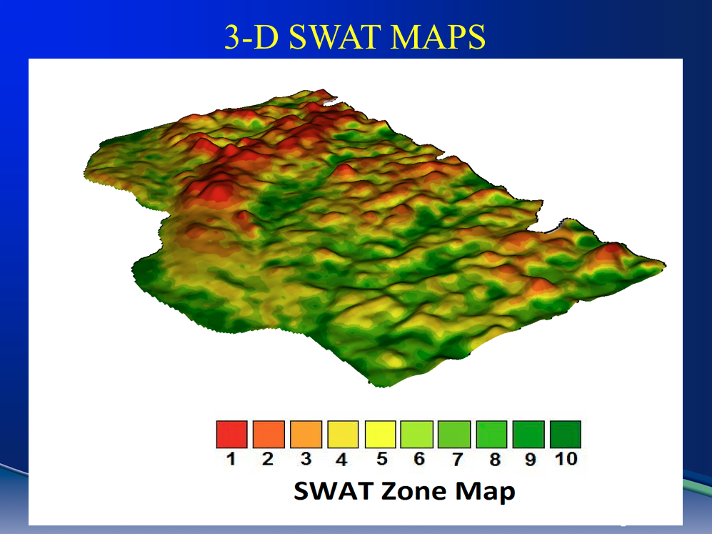
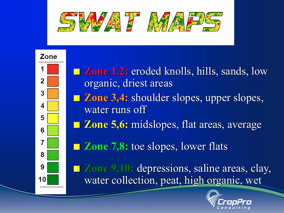
Our SWAT MAPS have ten Zones. Zone 1 is at the top– eroded knolls, sandier soils. As you go down, you get to your mid-slopes, and as you get to Zones 9 and 10, these will be depressions, high organic matter areas.

Typically, this is what you would see with an electrical conductivity map. Because it is in 3D, you can see all the water shedding areas throughout this field are low EC. This is what I would call fairly typical – areas that shed water -they’re typically coarser textured. Areas that are starting to collect water a little bit, these are mid-slope soils, so they have a slightly higher electrical conductivity, but it’s not a bad thing. Areas that are blue and purple on this map are areas of salinity. So, one challenge with salinity that we find is it’s nice to say you’re going to seed it down to grass and you’re going to tile it and all these things, but when they’re all spread, the little patches all throughout the field like this, it’s basically impossible, right? You’re farming through them. You’ve got to deal with them.

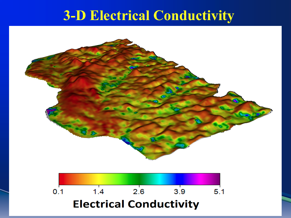
It is important to understand that you can never use EC as a layer on its own. You can get high EC on the tops of the hills and high EC and salinity in the low spots – two totally different things.

RTK elevation is a tremendously valuable piece of data but is useless as a zone map. You can have a depression at a high elevation that holds water while a knoll lower down sheds water. Elevation doesn’t know if it collects water or doesn’t collect water. It doesn’t know if it’s wet or dry. It doesn’t know if it’s a hill or a depression. You need a topography model.

We use 3D topography models as part of our SWAT Maps. Topography and elevation are not the same thing, but topography models themselves are still useless on their own. Why is that? Well, because all depressions are not the same. A depression can drain. A depression can flood, and a depression can be saline. Those aren’t all the same things. I don’t want to put those all into one zone.

We model where the water sits in this field. You can see the flow paths, where water is held in depressions. I don’t talk about it much, but if people are doing tile drainage or surface drainage, you need this type of modelling. You need RTK elevation. You need to map where all your depressions and flow accumulations are. You need to know where your salinity is because those are all things you want to fix.

You can also collect soil organic matter maps. The hills are low organic matter, and the places where water and erosion are accumulated is high organic matter. This isn’t rocket science, but it’s another map. Now, organic matter is useless on its own, too. So, there’s still all these problems using single-layer maps.

All of those layers are just base layers to build the model. So, here’s a final SWAT map where we have combined soil, water and topography layers together. We’ll make several different maps, and then the agronomist goes to the field and ground truths them. You soil test. You do expensive ground truthing to make sure you’re picking the right map for the field.

The most extreme hills are all in the Zone 1 – the lowest organic matter. Some of the smaller water shedding areas are Zone 3. All the midslopes are Zone 5 and 6. So, these are areas that are never too wet or too dry. You start collecting water as you go into 6 and 7. You have light salinity in Zone 9, and severe salinity is in the Zone 10. So, that’s all those layers together.

We treat soil potential maps or SWAT MAPS 100 per cent separate from biomass and yield maps. These are two totally different ways of collecting data and building the maps. The layers of maps we develop are for applying inputs in the soil. I don’t know how else you can go out there and apply inputs in the soil without having all those layers.

Prescription mapping

The second part of the equation is to get the fertilizer rates right using the SWAT maps. The goal is to get the fertilizer rates right for each area to provide the optimum return. We soil test these fields. We always make a ten-zone map because we love the resolution it gives us on the map, but it’s too expensive and too time-consuming to soil sample ten zones so we sample five zones. We lump Zones 1+2, 3+4, 5+6, 7+8 and 9+10 together. Our trucks have two different soil samplers in them, so we can do 24” cores at any depth. You’re zone sampling, based on soil, water, and topography.

Soil tests can be variable. In 2017, one of our agronomists kept five samples from each zone separate, and had them analyzed separately for P. Some zones were fairly uniform but others were very variable. Over all the zones, probably 30 per cent of the acres are extremely low in P, but as you get into Zones 9 and 10 it’s loaded with P, and there is salinity there, too.

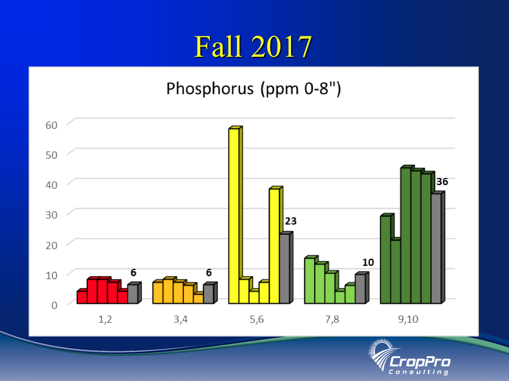
The farmers are always, constantly beating us up, “Well, prove to me that it pays. I want to see some research.” I say there’s a simple solution. Take all this phosphorous in Zone 9 and 10 where there’s no crop growing, put it up and gamble in all the higher more productive ground that is low on P. Put it back into your good ground.

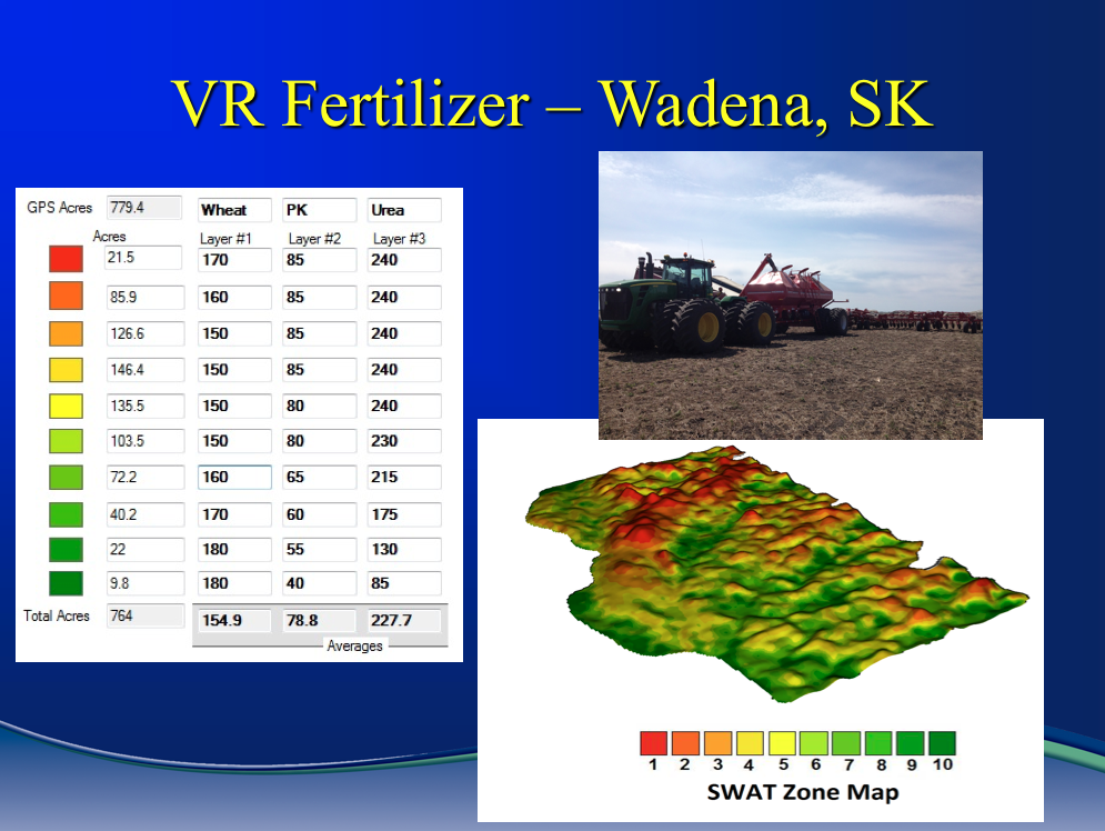
So, here’s just a prescription for this field: PK blend, very high phosphorous rates in all the Zone 1 to 4. Still very high rates, 80 lbs., in the midslopes and then cranked it right off to next to nothing down in the depressions Zones 9 and 10. Urea, even though we have ten different zones, we’re putting on high rates of urea in all the Zones 1 to 6, and cutting it right back in the depressions.

VR Seeding rates

About 95 per cent of what we do is variable rate fertilizer rates and seed rates. What do you do with variable rate seed? I’m going to use an example of wheat. We want to target thick plant stands in the Fusarium regions of western Canada — the Black soil zones and heavier moisture areas. We target plant stands of 30 plants per square foot. We’re trying to get more main stems for Fusarium and wheat midge control. We want uniform growth so we can target the correct timing for fungicide application.

So, what was the strategy? We put on the target seed rate in all the midslopes because it’s the most consistently established in this field. We put more seed on the hills, and quite a bit more in the depressions and salinity areas. This might be different for different fields or different areas.

We always do plant stand counts in the field. Basically we were able to achieve 30 plants per square foot in all the Zones except in the salinity where stands were 22 plants.

At the end of the year, this farmer is spraying all of his crops for Fusarium. When he goes to spray for Fusarium, he wants to see the hills and the depressions coming into maturity at the same time. At 30 plants per square foot the field is all main stems, and the whole field is consistent from hills to depressions. If it’s that consistent at fungicide staging, what do you think it’s like at harvest time, right? It’s more consistent. Seed growers, the conversation isn’t even yield. Most often, it’s about maturity and keeping the fields as even as possible because as soon as it’s ready to go, they want to get out there and get on that stuff and get it in the bin as soon as possible. So, everyone’s goals are slightly different.

More from the 2019 Soil Summit

Watch Cory Willness break down the difference between SWAT maps and other satellite or drone imagery as well as offer tips for growers looking to improve their variable-rate practices in his Speaker Spotlight video. To see other presentations and speaker spotlight videos, visit our archives for the 2019 Soil Management and Sustainability Summit.